A Drawing Nobody Can Query
Ask a process engineer which valves sit between a pump and a tank, and on many plants the answer starts with opening a PDF and tracing lines with a finger. The P&ID (piping and instrumentation diagram) holds that knowledge: every vessel, valve, instrument and pipe, and what connects to what. But on older plants it often exists only as an image, so the computer can show the drawing and nothing more.
What you want is the same drawing as data: components in one table, connections in another, or a graph where "what is upstream of this valve" is one query. I built pid-parser to do that conversion with a vision LLM, and measured it against ground truth until it was good enough to share.
Code: github.com/dzakybd/pid-parser (MIT) · Demo: huggingface.co/spaces/dzakybd/pid-parser
TL;DR
- What it is: an agent skill. Give it a P&ID image, get
graph.jsonplus SQL, CSV, GraphML and Neo4j Cypher. Install withnpx skills add dzakybd/pid-parser.- How: no GPU and no training. A vision LLM reads the drawing in two passes, symbols first and pipes second; small scripts tile it, check the graph and export it.
- How well: with gpt-6.1-sol, connection F1 is 0.80 on real sheets from the PID2Graph dataset and 0.83 on synthetic ones, at three to six minutes a sheet.
- Why it works: pipes run across the whole sheet, so the pipe pass always sees the whole sheet.
How It Works, Step by Step
The pictures below follow one synthetic sheet from PID2Graph through the pipeline. gpt-6.1-sol scored 1.00 on both symbols and connections for this sheet.
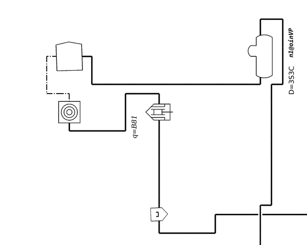
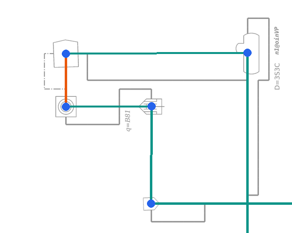
1. The drawing. The input is one P&ID sheet as an image, a scan or an export. Here is a part of it.
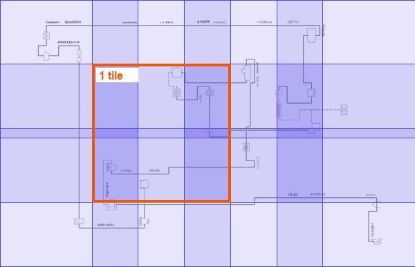
2. Tile it. A script cuts the sheet into overlapping crops of 1200 pixels and draws a pixel grid on them. The tiles overlap both across and down. Each neighbour shares at least 150 pixels, and because the script spreads the tiles evenly over the sheet, the real overlap is usually much larger: on the sheet below, 780 pixels across and 1250 down, in original pixels. It is the same idea as chunking a long document with overlap before you feed it to a model. A vision model shrinks a large image before it reads it, so on a whole sheet a valve a few dozen pixels wide turns into a smudge; in a crop it stays readable. The overlap is there for the same reason chunks overlap: a symbol cut in half by one tile's edge sits whole inside the next tile. The price is that a symbol near the middle of the sheet shows up in up to four tiles, and code has to merge those copies back into one.
Does a model as strong as gpt-6.1-sol still need the tiles? I measured the symbol pass alone both ways on all six sheets, scored against ground truth:
| Sheet | Whole sheet, 1 call: symbol F1 | Tiles: calls, symbol F1 |
|---|---|---|
| Real, dense (102 symbols) | 0.97 | 6 calls, 0.91 |
| Real (41 symbols) | 0.95 | 6 calls, 0.91 |
| Real (101 symbols) | 0.96 | 6 calls, 0.91 |
| Synthetic 1 | 0.98 | 12 calls, 0.88 |
| Synthetic 2 | 1.00 | 12 calls, 1.00 |
| Synthetic 3 | 1.00 | 12 calls, 0.98 |
On its own, the whole sheet won. Both ways found the same symbols; the tiles lost precision, because the overlaps produce duplicates the merge does not always catch. So I ran the full pipeline with a whole-sheet symbol pass. It was no better at the end: connection F1 0.61 against 0.75 on one real sheet and 0.85 against 0.84 on the dense one. The pipe agent revises the symbol list anyway, and it washed the head start out: it added ten symbols on one sheet and dropped thirteen on the other. Tiles stayed the default for three more reasons. The pipe pass zooms into the marked tiles. A 7000 by 4500 sheet was too big for the API to take in one image at all ("exceeding the limit of 30000 patches"). And with a smaller model, gpt-6-luna, tiling was the difference between finding a third of the symbols and finding most of them (symbol F1 0.33 against 0.81).
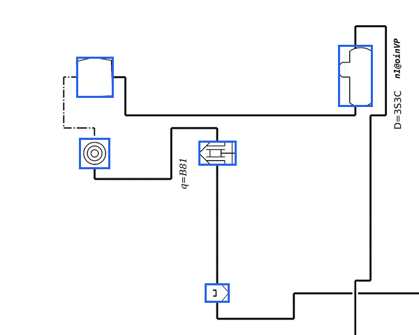
3. Symbols, one call per tile. For each tile the model lists every symbol it sees: its type (valve, pump, vessel, instrument and so on), the tag printed next to it, and its box. Boxes come back relative to the crop and code converts them to the original pixels, because a model can report positions in its own downscaled copy of the image instead of the original. Code then merges the duplicates from the overlaps.
4. Draw the ids. A script writes each symbol's id on the image. Now the model can say "s10 connects to s11" instead of describing where things are, which it does much less reliably.
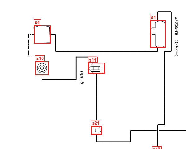
5. Pipes, on the whole sheet. An agent opens the overview and the marked tiles and follows every line from id to id. A valve in the middle of a line splits it into two edges. Where three or more pipes meet, it adds a junction node. Dashed instrument lines become signal edges.
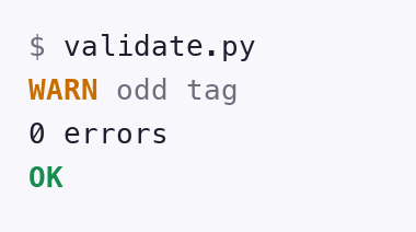
6. Validate. A script checks the graph with plain rules: unknown ids, edges to nothing, isolated valves, junctions with fewer than three branches, tags that do not look like tags. It has no answer key and no model in it; it only catches things that cannot be right on any P&ID. The agent goes back to each flagged spot and fixes what is wrong. Here the only warning was a tag, because synthetic sheets use random strings as tags.
7. Export. The graph goes out as SQL, CSV, GraphML and Cypher.
| File | Load it with |
|---|---|
pid.sql | sqlite3 pid.db < pid.sql or psql -f pid.sql |
nodes.csv, edges.csv | any spreadsheet or COPY |
graph.graphml | NetworkX, Gephi, yEd |
graph.cypher | cypher-shell -f graph.cypher (Neo4j) |
What You Can Ask It
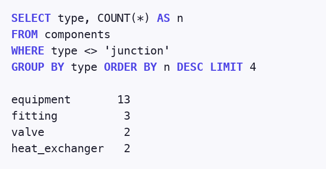
The two formats answer different questions. SQL is for counting and filtering: how many of each component, which valves have no tag, which lines carry a given line number. Here are the four most common component types on the sheet above:
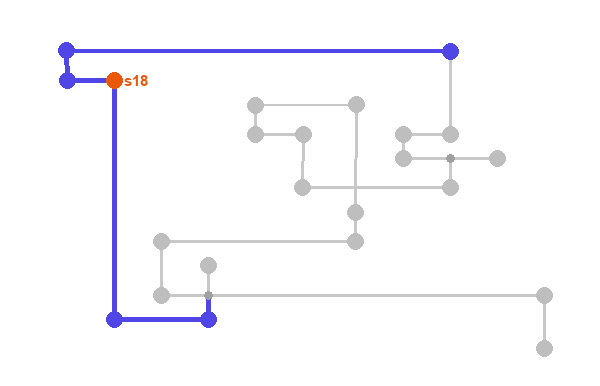
The graph is for "what connects to what". Pipes meet at junctions before they reach equipment, so in SQL a valve's direct neighbours are often just junction points, and following a pipe means one self-join per hop. In Neo4j one pattern walks through them. This asks what the check valve reaches within three pipe hops:

I loaded the exports into SQLite and into a Neo4j 5 container to check that both work, and the showcase Space has three converted sheets with every file to download.
Two Ways to Run It: a Skill or a Deep Agent
Everything lives in one repository, dzakybd/pid-parser (MIT), with a live demo in the Hugging Face Space:
pid-parser/
├── skills/pid-parser/   the skill: SKILL.md + tile.py, mark.py, validate.py, export.py
├── agent/run.py         the LangChain Deep Agents version, which runs the same skill
├── eval/                the ground-truth scorer and the comparison scripts
└── space/               the Hugging Face showcase
The skill folder is the single source of truth. The Deep Agents version does not copy its instructions; it loads the same SKILL.md, so a fix to the skill reaches both.
As a skill in Claude Code, Codex or another harness
npx skills add dzakybd/pid-parserThen ask: "Use the pid-parser skill to parse drawing.png." The agent reads SKILL.md and runs the scripts. They only need Python and Pillow. This is the easiest path if you already use one of these tools.
As a LangChain Deep Agent, on a ChatGPT sign-in
For a pipeline you run from your own code, agent/run.py builds the same flow with LangChain Deep Agents. It runs on a ChatGPT subscription through the sign-in with ChatGPT provider, so no OpenAI API key is needed.
| Piece | Version |
|---|---|
| Python | 3.12 |
deepagents | 0.7.25 |
langchain-openai | 1.7.2 (for _ChatOpenAICodex, still experimental) |
langchain-core / langgraph | 1.6.10 / 1.2.15 |
| Model | gpt-6.1-sol, reasoning effort low |
git clone https://github.com/dzakybd/pid-parser
cd pid-parser && uv sync

# once: sign in with your ChatGPT account
uv run python -c "from langchain_openai.chatgpt_oauth \
  import login_chatgpt; login_chatgpt()"

mkdir -p work/skills
cp -R skills/pid-parser work/skills/ && cp drawing.png work/
uv run python agent/run.py work \
  --model gpt-6.1-sol --effort low --tiled
The core of run.py is short. Code runs the symbol pass with plain structured-output calls, one per tile, writes graph.json, and then hands a Deep Agent the rest. Simplified from agent/run.py:
from deepagents import create_deep_agent
from deepagents.backends import LocalShellBackend
from langchain_openai.chat_models.codex import _ChatOpenAICodex

model = _ChatOpenAICodex(
    model="gpt-6.1-sol", reasoning={"effort": "low"}
)

# Pass 1 in code: one structured-output call per tile,
# then merge the duplicates from the overlaps
symbols, w, h = tile_symbols(model, "work/tiles")
graph = {"nodes": merge(symbols, w, h), "edges": []}
# ...saved as work/graph.json

# Pass 2 onward: an agent that loads the same SKILL.md
agent = create_deep_agent(
    model=model,
    system_prompt=SYSTEM,
    skills=["work/skills"],  # finds skills/pid-parser/SKILL.md
    backend=LocalShellBackend(  # real files and a real shell
        root_dir="work", virtual_mode=False
    ),
)
task = ("Steps 1-2 are done. Mark the ids, add the connections, "
        "validate and fix, then export.")
agent.invoke({"messages": [{"role": "user", "content": task}]})
Deep Agents supplies the parts I did not want to write: it loads the skill, gives the model file and shell tools so it can open images and run the scripts, and keeps the loop going until the export exists. Two settings mattered. virtual_mode=False with real absolute paths in the task, or the agent could not find the skill's scripts. And the split itself: code does the symbols, the agent does the pipes. The section on the pipes below shows what happened when one agent did everything.
I picked a skill over a trained model on purpose. A trained detector, like the Relationformer model published with PID2Graph, needs labelled data, a GPU and retraining when the drawing style changes. A skill is a text file and four scripts, and it gets better when the model does.
How I Measured It
There are two kinds of checking in this project, and they are easy to mix up:
- The validator in step 6 runs every time you use the skill. It knows nothing about the right answer. It applies rules that hold on any P&ID, so it catches broken graphs, not wrong ones. A pipe drawn to the wrong valve passes it.
- The scores below come from ground truth. I ran the skill on sheets whose correct graph is known and compared the two with a deterministic script. No LLM judges anything.
I did not use an LLM as the judge on purpose. A second vision model reading the same drawing shares the same blind spots: if one misses a faint line, the other can miss it too and call the answer right. When a real answer key exists, it is the better judge.
PID2Graph has P&ID sheets with the true graph for each one. I used real sheets from its OPEN100 part and three synthetic ones, and pulled only those files out of the 9.3 GB archive with HTTP range requests.
- Symbols: each predicted box is matched one-to-one to a true symbol if its centre falls close enough to it. Symbol F1 says how many were found and how many were made up.
- Connections: two symbols count as connected when they sit on the same pipe network. Connection F1 compares those pairs with the truth. This is the hard number.
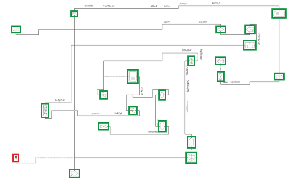
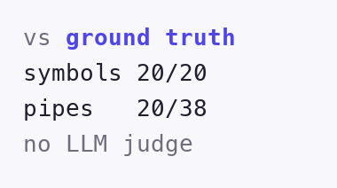
Here is what that looks like on a sheet the pipeline did not get right. Every predicted symbol is drawn on the drawing: green when it matched a symbol in the answer key, red when the answer key has nothing there. All 20 true symbols were found, plus one extra. The pipes were worse: 20 of the 38 true symbol pairs. That number drops fast: a single missed pipe can split a network in two, and every pair across the split then counts as missed.
Before trusting the scorer I tested it: a perfect answer built from the ground truth scores 1.0, dropping every fifth symbol lowers recall as expected, and shifting every box by 3% of the sheet's diagonal makes symbol F1 collapse.
| Setup | Real sheets: symbol F1 | Real sheets: connection F1 | Synthetic: connection F1 | Time a sheet |
|---|---|---|---|---|
| Deep Agents, gpt-6.1-sol, low effort | 0.91 | 0.80 | 0.83 | 3 to 6 min |
| Deep Agents, gpt-6.1-sol, medium effort | 0.92 | 0.81 | 4 to 5 min | |
| Claude Code, Opus | 0.78 | 0.59 | 0.85 | 3 min |
| Codex, gpt-6-sol | 0.73 | 0.49 | 0.65 | 3 min |
The gpt-6.1-sol rows ran on two real sheets, the Claude Code and Codex rows on three, so read the real-sheet columns as a rough comparison. I ran each setup once per sheet, and the same setup can move by up to 0.2 between runs. Low and medium effort scored the same within that noise, so low is the default.
Why the Pipes Need the Whole Sheet
Before this design I tried reading the pipes tile by tile, then joining the pieces: by shared symbols, by the printed line number, and by carrying each pipe's loose end into the next tile. Every version scored lower than reading the pipes with the whole sheet in view. A pipe that leaves one tile has to be matched to the right piece in the next one, and one wrong match merges two pipes that are separate on the drawing.
Does a model as strong as gpt-6.1-sol still need code to run the symbol pass? I ran it both ways, once per sheet. On the simpler real sheet it made no real difference: connection F1 0.86 when the agent ran the whole skill itself, 0.75 with code running the symbol pass, inside the run-to-run noise. On the dense sheet it mattered: 0.37 against 0.84. Symbols came out about the same both ways; the pipes did not. Left with the whole job, the agent finished the dense sheet in 8 tool calls. With the symbols already done, it spent 21 on the pipes alone. Handing the symbol pass to code leaves the agent its full effort for the hard part.
A group at Imperial College London reached the same split independently. Their ESCAPE 36 paper reads the drawing first and rebuilds the topology in a second step, and that raised edge accuracy from 55.6% to 80.6% on their first case study.
What It Does Not Do Yet
- Tags are not scored. PID2Graph has no tag text, so I checked tags by eye only. Treat them as a draft to review.
- A handful of sheets is not a benchmark. The real-sheet numbers for gpt-6.1-sol come from two sheets. They show the method works; they do not prove it on your drawings.
- Dense sheets are the weak spot. Long headers that connect twenty symbols are where every setup lost the most.
- It depends on the model. It got better with no change from me when the model improved, and a weaker model will do worse.
Try It
- Install the skill:
npx skills add dzakybd/pid-parser, then ask your agent to parse a drawing. - Browse three converted sheets with downloads in the showcase Space.
- Read the code, the scorer and the Deep Agents runner: dzakybd/pid-parser.
If you work with P&IDs: how does your team turn drawings into data today, by hand, with a vendor tool, or not at all? I would like to know where this would and would not fit.
References
- PID2Graph dataset (CC BY-SA 4.0) and its paper, arXiv 2411.13929. The drawing pictures in this post come from its synthetic part.
- Zhu, Duong, Vyas and Mercangöz, From P&ID Drawings to Process Graphs: A Multimodal Language Model Approach, ESCAPE 36 (2026)
- LangChain Deep Agents and sign in with ChatGPT
- skills CLI for
npx skills add - My code and showcase: dzakybd/pid-parser, Hugging Face Space